We now formulate power-demand routing in geo-distributed systems as an optimization problem, in which we wish to assign client requests to clusters minimizing the total operating cost of a system (performance, network costs, and energy costs).

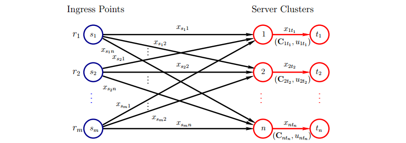
Fig.4.1: A network for power-demand routing

We show a network flow model of power-demand routing (see   : 1  for more details on network models). We are given a network, depicted in Figure 4.1, with \(m\) ingress points in blue, (the source - the supply nodes), where client requests arrive, denoted by \(s_i, i = 1, . . . ,m\). For each ingress point \(s_i, i = 1, . . . ,m\) the number of requests is specified by nonnegative integer number \(r_{s_i}\). The ingress points may represent IPS’s, network prefixes or some other groupings. These requests have to be distributed among n server clusters (the sinks) denoted by \(t_i, j = 1, . . . , n\). The requests flow on the server cluster arcs \( (j, t_j ), j = 1, . . . , n\) (see Figure 4.1, in red). The clusters model groups of servers together with their support infrastructure. Each server cluster arc \((j, t_j )\) has an associated cluster capacity \(u_{jt_j} , j = 1, . . . , n\), that denotes the maximum number of requests the server cluster can service. The decision variables in this network model are arc flows. The flow on arc \((s_i, j)\) represented by decision variable \(x_{s_i j}\) is the number of requests sent from ingress point si to server cluster \(j\); the flow on arc \((j, t_j)\) represented by decision variable \(x_{jt_j}\) is the request volume assigned to server cluster \(j, i = 1, . . . ,m\), \(j = 1, . . . , n\), i.e. the number of requests, server cluster \(j\) must service. The optimization process during the course of determining an optimal solution, represented by the decision variables, in this network model must take into account a number of cost criteria, such as energy costs, system performance costs, network costs, etc., modeled by \(C_{jt_j} (x_{jt_j})\), a vector of cost functions assigned to server cluster arc \((j, t_j)\) depending on flow \(x_{jt_j}\) on \((j, t_j)\). We describe cost functions in details later on. Thus, the optimization is a multiobjective network optimization.

We consider the multiobjective network optimization subject to the following assumptions.

Centralized location: A centralized location is assumed, i.e. a place where all the information about the network model is collected. Then after computing an optimal solution \(x_{s_i j}\), the optimal request flow \(x_{s_i j}\) is pushed into the network through the arcs \((s_i, j)\).

Discrete time process: The PDR is modeled as a discrete time process. Namely, the time horizon is divided into equal time intervals. At the beginning of each time interval an optimal request flow \(x_{s_i j}\) is computed. Then the flow of the requests is immediately pushed into the network. Obviously, such traffic optimization can be performed when the time needed for determining an optimal request flow \(x_{s_i j}\) and deploying them into the network (pushing the flow on new routes \((s_i, j))\) is smaller than the length of the time interval (the length of the time interval can be one hour). It is assumed the optimization process is a memory less one (see   : 2  for discussion).

Feasibility: To ensure feasibility of the above network model the total incoming request traffic and the total capacities must fulfill the inequality: \(\sum^{m} _{i=1} {r_{s_i}} \le \sum^{n} _{j=1} {u_{jt_j}}\). Now, cluster capacities \(u_{jt_j}, j = 1, . . . , n\), denote the maximum numbers of requests, the clusters can service before they become overload in one time interval.

Replication and homogeneous requests: It is assumed that the system we optimize is fully replicated one with homogeneous requests. Therefore, any request can be sent to any cluster server, see   : 2  for for a optimization model extension that deal with partially replicated systems.

Precisely known parameters: The all input parameters such as the number of requests that arrive at ingress points, electricity prices are precisely known at the beginning of each time interval. One can takes parameter uncertainty into account but then it leads to an optimization model whose solving is time consuming, e.g. stochastic   : 3  and robust   : 4  models.

Network model: It is assumed that all ingress points are connected with all cluster servers - a fully connected network model. Since we assume that each ingress-to-cluster link, arc \((s_i, j)\), is over-provisioned, its capacity is not specified. To model delays in our network model, we use average latency \( l_{s_i j}\) that can be determined by adding network and cluster means. Namely, \[ l_{s_i j}(x_{s_i j}) = \delta_{s_i j} + \pi_{jt_j} (x_{jt_j}), \] where \(δ_{s_i j}\) is the mean network latency (round-trip time, in \(ms\)) of ingress-to-cluster link \((s_i, j), \pi_{jt_j }(x_{s_i j})\) is the mean processing delay in the cluster j, i.e. the average time, in \(ms\), between a moment when a request arrives to cluster \(j\) and a moment when a response leaves the cluster, when the cluster load is \(x_{jt_j}\) requests.