The effectiveness of the disk power management system can be improved by modifying disk layout of the striped data files . We use the following abstractions for disk layout optimisation.

File striping: A large amount of data is divided into small fragments (stripes) stored on a group of separate disks in a round-robin fashion. We assume that we have a set of disks \( \{ d_0, d_1, \ldots, d_m \}\). For each data array contained in a file we can specify the following parameters:

• start disk -- the disk from which the array is started to get stripped
• stripe factor -- the number of disks used to stripe the data
• stripe size -- the size of single stripe

The following figure illustrates the layout of the files \(U\) and \(V\) with the (start disk, stripe factor, stripe size) parameters set to \( (d_0,6,S) \) and \( (d_4,3,2S)\), respectively, on the set of eight disks \( \{d_0,\ldots,d_7\} \):

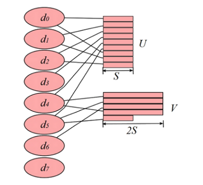
Fig. 7.2/1

We assume that each disk contains a timer-based power management. Each disk can be in one of the following states:

• Active
• Idle
• Standby

Transitions between the states are illustrated by the following diagram:

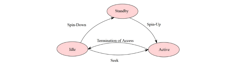
Fig. 7.2/2

Disk is idle between the periods of activity, when its data are being accessed. If the disk remains in an idle state for a certain amount of time, it is spun down to the standby mode. When a new request to the disk is made it has to resume the active mode by spinning up. Spinning up takes both extra time and extra energy. Therefore the number of such transitions should be minimized.

If we consider the energy consumption alone, then the optimal solution would be placing all data on a single disk and switching off all the remaining disks. However, this would cancel the performance benefits of disk striping -- all the I/O requests would have to be served sequentially by a single disk. We would like to save as much energy as possible without significant deterioration of performance.

The disk layout detection algorithm is a profile driven heuristics. The application code is instrumented and profiled using standard input set. The inserted instrumentation code records information about disk accesses, for each of its data arrays, in the form of the array access sequence. This array access sequence is an input for layout optimizer, which computes disk layouts.

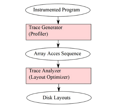
Fig. 7.2/3

The array access sequence is of the form \( (A_1,A_2,\ldots,A_n) \). Each access \( A_i \) has the form \( (X,a,t) \), where

• \( X \) is identifier of disk-resident array
• \( a \) is the offset of the accessed element within the array
• \( t \) is the time-stamp of the access (the time since the start of the program after excluding the time spent on I/O operations).

Note that each conflict slows down the program execution, since one of the conflicted accesses is delayed by the other. Thus, the goal of layout optimisation is to find, for all arrays, the triples (start_disk, stripe_factor, stripe_size) that reduce the energy consumption, while minimizing the number of conflicts.

The exhaustive search for optimal solution is generally not possible due to a large number of possible configurations of parameter values even in modest sets of disks and data arrays. Therefore we consider the following heuristics:

1. First, determine the stripe factor for each array.
2. Then, determine the stripe size for each array.
3. Then, determine the starting disk for each array.

The first two steps attempt to minimize the intra-array conflicts. The third step positions the arrays on the disk system in such a way that the number of inter-array conflicts is minimized.

Consider the following example code:

The size of each element of each array is one byte. The system supports stripe sizes: 256B, 512B, 1024B, and 2048B. There are six disks. The response time of each disk is 5 ms. For all loops L0, L1, and L2, each loop iteration takes 10 ms.

To avoid intra-array conflicts, the stripe-factors for \(X\), \(Z\), and \(Y\) must be 2,3, and 1, respectively.

For stripe sizes 256B, 512B, 1024B, and 2048B, the numbers of intra-array conflicts, for array \( X \) in loop L1, are 2048, 2048, 0, and 1024, respectively. Thus we select stripe size 1024B for array \( X \). Similarly, stripe size 256B is selected for array \( Z \). Stripe size for \( Y\) does not need to be considered.

The starting disk for each array are selected to minimize the inter-array conflicts. There example of such layout is:
Layout 1:

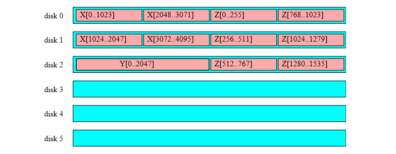
Fig. 7.2/4

The following layout also minimizes the number of conflicts:
Layout 2:

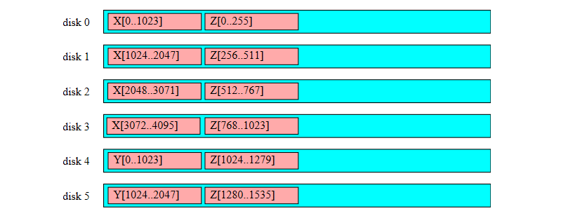
Fig. 7.2/5

However, we also have to consider the transitions between the power-down and active states of the disks that consume additional energy and induce some additional delays:
Disk power states for Layout 1:

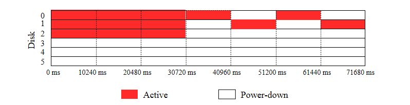
Fig. 7.2/6

Disk power states for Layout 2:

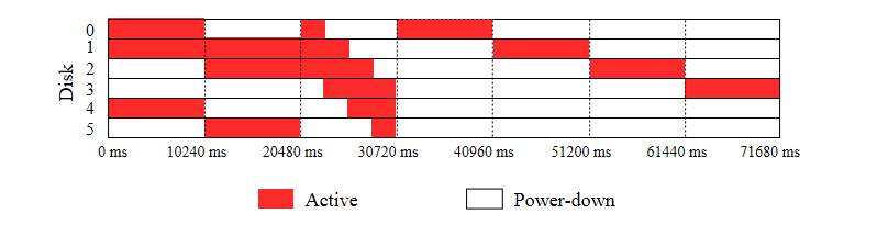
Fig. 7.2/7

It is clearly visible that the number of power states transitions is lower for Layout 1 and, hence, this layout should be selected.

1. What is file striping and why is it used?
2. Why should we try to minimize the number of disks' power-state trasitions between power-off and active states?
3. Try to implement any simulator of the heuristic discussed above for explicitely provided array input sequence.